


Random forest, an ensemble method
The random forest (RF) model, first proposed by Tin Kam Ho in 1995, is a subclass of ensemble learning methods that is applied to classification and regression. An ensemble method constructs a set of classifiers—a group of decision trees, in the case of RF—and determines the label for each data instance by taking the weighted average of each classifier’s output.
The learning algorithm utilizes the divide-and-conquer approach and reduces the inherent variance of a single instance of the model through bootstrapping. Therefore, “ensembling” a group of weaker classifiers boosts the performance and the resulting aggregated classifier is a stronger model.
Random decision forest is a modification of bagging – bootstrap aggregating, proposed by Leo Breiman in 2001—that assembles a large collection of decorrelated trees on randomly selected features[1]. The ``number of trees`` composing the forest is related to the model’s variance, while the ``depth of the tree`` or ``maximum number of nodes that each tree is consisted of`` is associated with the irreducible bias present in the model.

RF has a number of advantages: It is very fast to implement and execute (runs efficiently on large datasets), one of the most accurate learning algorithms, and resistant to overfitting and outliers[2]. The performance of RF is similar to but more robust than that of gradient boosted decision trees (GBDT), another subclass of tree ensemble methods. Furthermore, since RF has fewer hyperparameters than GBDT, it is easier to train and tune. As a consequence, RF is very popular and is supported in various languages such as R and SAS, and many packages in Python including scikit-learn and TensorFlow.
Tensor_Forest estimator [Note: only compatible with TF 1.2.0]
TensorFlow has recently included support for RF in the contributed code base – tf.contrib – through a module named tensor_forest (defined in https://github.com/tensorflow/tensorflow/blob/master/tensorflow/contrib/tensor_forest/__init__.py, note that the link to tensor_forest on the official TensorFlow website directs the user to the branch with most recent version and not to master branch). There is significant modification to tensor_forest in version 1.3.0 from version 1.2.0 and the code structure and parameters to be discussed complies with version 1.2.0.
Structure of Tensor_Forest[3]
The following modules should be imported to use tensor_forest:
from tensorflow.contrib.learn.python.learn import metric_spec
from tensorflow.contrib.learn.python.learn.estimators import estimator
from tensorflow.contrib.tensor_forest.client import eval_metrics
from tensorflow.contrib.tensor_forest.client import random_forest
from tensorflow.contrib.tensor_forest.python import tensor_forest
The initial step to running RF in TensorFlow is constructing the model. To build an RF estimator, first specify the hyperparameters of the RF as the following:
hparams = tensor_forest.ForestHParams(
num_classes=NUM_CLASSES,
num_features=NUM_FEATURES,
num_trees=NUM_TREES,
max_nodes=MAX_NODES,
min_split_samples=MIN_NODE_SIZE).fill()
Each of the hyperparameters for tensor forest mentioned above is described below:
``num_classes``: The number of possible classes for labels
``num_features``: The number of features. Either ``num_splits_to_consider`` or ``num_features`` should
be set; according to the code contributors of tensor_forest, the model is more accurate
when ``num_splits_to_consider`` == ``num_features``[4].
``num_trees``: The number of trees to build for taking the mode [for classification] or mean [for
regression] of predictions. Trees are “notoriously noisy” so they “benefit greatly from averaging”[5]. The more trees consisting the forest, the lower the variance of the model and hence the more accurate the results. However, there is a trade-off between output performance and speed of execution. Using a large number of trees means more computational cost and could significantly slow down the code. Usually, after a certain number of trees, model performance plateaus and improvement is negligible[6].
I like to build a five-tree forest to test my code for debugging purposes, a 100-tree for getting an initial feel for accuracy, precision, recall, auc, etc., and a 500-tree for a final model that does not need major adjustments. Generally, using a 1000-tree model does not significantly boost performance from a 500-tree forest.
*Default: 100
The following two hyperparameters determine tree depth in a forest. Limiting tree depth does not give any additional bonus other than limiting computing time and is not recommended[7]. Larger depth means smaller bias. When trees “grow sufficiently deep, [they] have relatively low bias”[8].
``max_nodes``: The maximum number of nodes allowed for each tree. A larger number of ``max_nodes``
allows for deeper trees.
*Default: 10000.
``min_split_samples``: “The minimum number of samples required to split an internal node” according to
SKlearn[9]. ``min_split_samples`` is related to minimum node size. The fewer number of samples required to split a node, the deeper the tree can grow.
*Default: 5
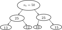
[10]Visualization 1: A tree with minimum node size of 10.
Then, determine the type of graph to be used with RF; there are two types of graphs: The default RF graph [``RandomForestGraphs``] and the training loss graph [``TrainingLossForest``][11]. For the prior, user can upweight the positive instances, usually for imbalanced datasets, by passing in a weights vector.
[Note: ``SKCompat`` is the scikit-learn wrapper for TensorFlow[12]. ``model_dir``should be a directory where the RF and the log file for tensorboard visualization is saved.]
If the RF graph is selected:
To specify an upweight:
graph_builder_class = tensor_forest.RandomForestGraphs
est = estimator.SKCompat(random_forest.TensorForestEstimator(
params,
graph_builder_class=graph_builder_class,
model_dir=MODEL_DIRECTORY,
weights_name=’weights’))
Or keep the default of 1:1 weighting of positive to negative data points:
graph_builder_class = tensor_forest.RandomForestGraphs
est = estimator.SKCompat(random_forest.TensorForestEstimator(
params,
graph_builder_class=graph_builder_class,
model_dir=MODEL_DIRECTORY))
In the case of training loss forest, training loss calculated from the default loss function [``log_loss``] or a specified loss function is used to adjust the weights[13].
Use the default ``log loss`` as the loss function:
graph_builder_class = tensor_forest.TrainingLossForest
Or specify a loss function to be used in the training loss graph[14]:
from tensorflow.contrib.losses.python.losses import loss_ops
# valid loss functions are:
#["absolute_difference",
#"add_loss",
#"cosine_distance",
#"compute_weighted_loss",
#"get_losses",
#"get_regularization_losses",
#"get_total_loss",
#"hinge_loss",
#"log_loss",
#"mean_pairwise_squared_error",
#"mean_squared_error",
#"sigmoid_cross_entropy",
#"softmax_cross_entropy",
#"sparse_softmax_cross_entropy"]
def loss_fn(val, pred):
_loss = loss_ops.hinge_lss(val, pred)
return _loss
def _build_graph(params, **kwargs):
return tensor_forest.TrainingLossForest(params,
loss_fn=_loss_fn, **kwargs)
graph_builder_class = _build_graph
Finally, construct the RF estimator with the previously specified hyperparameters and graph. est= estimator.SKCompat(random_forest.TensorForestEstimator(
hparams,
graph_builder_class=graph_builder_class,
model_dir=MODEL_DIRECTORY))
After the RF has been constructed, fit the model to training data via the ``fit`` method.
For RF graph with upweight specified*:
est.fit(x={‘x’:x_train, ‘weights’:train_weights},
y={‘y’:y_train},
batch_size=BATCH_SIZE,
max_steps=MAX_STEPS)
*Note: `weights` should be the same key as the one passed into ``TensorForestEstimator`` earlier.
``train_weights`` should be dimension: (number of samples, )
For default 1:1 weighting or training loss forest:
est.fit(x=x_train, y=y_train
batch_size=BATCH_SIZE,
max_steps=MAX_STEPS)
To evaluate results outputted by the model, identify the desired metrics and pass them to the ``evaluate`` function[15].
# other metrics include:
# true positives: tf.contrib.metrics.streaming_true_positives
# true negatives: tf.contrib.metrics.streaming_true_negatives
# false positives: tf.contrib.metrics.streaming_false_positives
# false negatives: tf.contrib.metrics.streaming_false_negatives
# auc: tf.contrib.metrics.streaming_auc
# r2: eval_metrics.get_metric('r2')
# precision: eval_metrics.get_metric('precision')
# recall: eval_metrics.get_metric('recall')
metric = {‘accuracy’:metric_spec.MetricSpec(eval_metris.get_metric(‘accuracy’),
prediction_key=eval_metrics.get_prediction_key(‘accuracy’)}
If upweight is given:
model_stats = est.score(x={‘x’:x_test, ‘weights’:test_weights},
y={‘y’:y_test},
batch_size=BATCH_SIZE,
max_steps=MAX_STEPS,
metrics=metric)
for metric in model_stats:
print(‘%s: %s’ % (metric, model_stats[metric])
For default weighting and training loss forest:
model_stats = est.score(x=x_test, y=y_test
batch_size=BATCH_SIZE,
max_steps=MAX_STEPS,
metrics=metric)
for metric in model_stats:
print(‘%s: %0.4f’ % (metric, model_stats[metric])
For the predicted label and probability of every class for each data instance:
[Note: ``predicted_prob`` and ``predicted_class`` are numpy arrays that preserves ordering of the original input]
Upweight specified:
predictions = dict(est.predict({‘x’:x_test, ‘weights’:test_weights}))
predicted_prob = predictions[eval_metrics.INFERENCE_PROB_NAME]
predicted_class = predictions[eval_metrics.INFERENCE_PRED_NAME]
Default weighting and training loss forest:
predictions = dict(est.predict(x=x_test))
predicted_prob = predictions[eval_metrics.INFERENCE_PROB_NAME]
predicted_class = predictions[eval_metrics.INFERENCE_PRED_NAME]
Lastly, spin up tensorboard through terminal to visualize the training process and TensorFlow graph:
The directory previously passed to ``model_dir`` should be given.
$ tensorboard --logdir="./"
Open http://localhost:6006/ or the link from running the command above in the browser to view tensorboard.
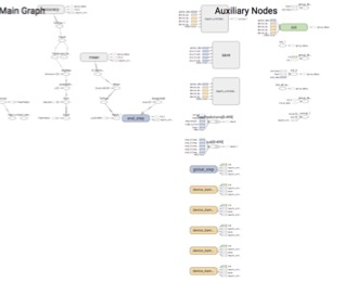
Visualization 2: Tensorboard for tensor_forest
A comparison between TensorFlow and scikit-learn
Currently, TensorFlow and scikit-learn are both very popular packages, each with teams of experts contributing and maintaining the code base, a myriad of tutorials on code usage online and in print, coverage of most machine-learning algorithms. However, these two modules are not aimed at the same tasks.
scikit-learn
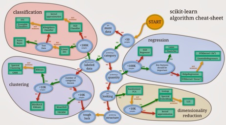
Visualization 3: Scikit-learn’s flowchart on selecting the right estimator[16]
Scikit has long being regarded as the “de facto official Python general machine learning framework”[17]. Itoffers a comprehensive code base of machine-learning algorithms that belong to various categories: classification, regression, clustering, dimensionality reduction, etc[18]. Those well-packaged algorithms equip users with off-the-shelf access to easy and quick analysis on the dataset. As an example, sklearn includes an RF module that can be deployed to datasets with only a few lines:
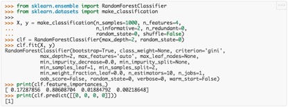
Visualization 4: An RF model implemented with scikit-learn[19]
Besides its effortless-to-use nature and standardized API, scikit-learn is also extraordinarily well-documented. For each library, there are pages dedicated to not only detailing the interface, input parameters, and output format, but also demonstrating the code usage with carefully constructed examples. Using sklearn’s RF module as a specific illustration again:
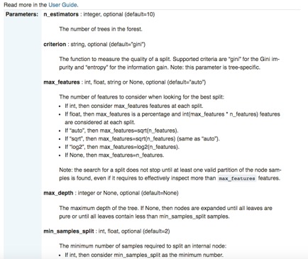
Visualization 5: Scikit-learn’s thorough description of each input parameter for ``RandomForestClassifier``[20]
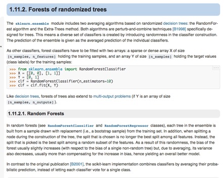
Visualization 6: Scikit-learn’s comprehensive account of the structure of an RF module[21]
While scikit-learn has numerous prominent advantages such as “syntactical brevity”[22], it does have one particular shortcoming: sklearn does not and will not support GPU in the near future[23]. “GPU support will introduce many software dependencies and introduce platform specific issues. [...] Outside of neural networks, GPUs don’t play a large role in machine learning today”, according to sklearn’s official website. On the other hand, TensorFlow’s native support for GPU particularly suits it for deep learning.
TensorFlow
The power of TensorFlow shines from its scalability to “train[ing] deep neural networks on GPUs[ and] possibly on clusters of multiple machines”[24], and the amount freedom granted to users in assembling their own deep learning algorithms. Users specify not only what type of model is utilized, but also how it is implemented by using the primitives provided by the framework[25]. They define exactly “how [...] data should be transformed [and] what loss function should the model optimize”[26]. In addition, TensorFlow is highly flexible and portable; it is available on extensive platforms – including Ubuntu, Mac OS X, Windows, Android, iOS – and a variety of languages, such as Python, Java, C, Go[27]. Although it seems especially attractive with the scalability and integrability, TensorFlow’s complicated code structure, mysterious error messages, and in some cases – poorly documented modules overburden the debugging process. Hence, utilizing TensorFlow for “most practical machine learning tasks” is probably overkill[28].
The solution: Scikit flow
[https://github.com/tensorflow/tensorflow/tree/master/tensorflow/contrib/learn/python/learn]
Scikit flow (SKFlow) is introduced as a solution to the scikit-TensorFlow dilemma: It harnesses the “modeling power of TensorFlow by channeling the syntactical brevity of scikit-learn”[29]. SKFlow is an official project developed by Google that provides a simplified high-level wrapper for TensorFlow[30].
A three-layer neural network with 10, 20, and 10 hidden units respectively can be implemented with four lines in SKFlow:
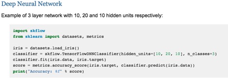
Visualization 7: Deep Neural Network in SKFlow[31]
Or building a custom model with SKFlow with around 10 lines of code:
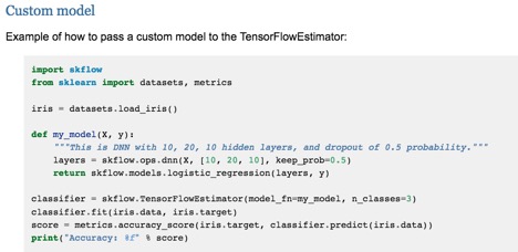
Visualization 8: Creating a custom model with SKFlo